Reversible optimisers

This post touches on a curious property of some common optimisers used by the machine learning community: reversibility.

I tend to hate reading through lengthy introductions, so let’s just dive in with an example. Take gradient descent with momentum, this has the following form \begin{align} \mu_{t+1} &= \alpha \mu_t + \nabla_{x} f(x_{t}) \newline x_{t+1} &= x_t - \lambda \mu_{t+1}. \end{align} Here $x_t$ denotes the optimisation variable, or position, $x$ at time $t$, $\mu$ is the associated momentum, and $0 < \alpha < 1$ & $\lambda > 0$ are metaparameters, which govern the dynamics of the descent trajectory. I use the term metaparameters, instead of hyperparameters, to distinguish that they are part of the optimiser and not the model, even though some would nowadays say that the optimiser is in fact part of the model, implicitly regularising it.

Anyway, interestingly we can reverse these equations, given the state $[x_{t+1}, \mu_{t+1}]$ as \begin{align} x_t &= x_{t+1} + \lambda \mu_{t+1} \newline \mu_{t} &= \frac{1}{\alpha} \left ( \mu_{t+1} - \nabla_{x} f(x_{t}) \right). \end{align} This seemingly arbitrary property is useful from a practical standpoint.

Memory efficiency

An oft-lauded property of reversible systems is that we do not have to store intermediate computations, since they should be easily reconstructed from the system’s end-state. Typically for reverse-mode differentiation to work (i.e. backpropagation), we have to store all the intermediate activations in the forward pass of a network. This has memory complexity, which scales linearly with the size of the computation graph. If we can dynamically reconstruct intermediate activations during the backward pass, then we instantly convert this linear memory complexity to a constant, which enables us to build (in theory) infinitely deep networks.

Momentum is additive coupling

Indeed, if you look a little closer at the momentum equations, then you may spot that they resemble an additive coupling layer. Here we have that a state, split into two parts $x$ and $\mu$ (to mimic the momentum optimiser notation), is reversible with the following computation graph \begin{align} \mu_{t+1} &= \mu_t + g(x_t) \newline x_{t+1} &= x_t + h(\mu_{t+1}) \end{align} To make a direct comparison, $g(x) = \nabla_x f(x)$ and $h(x) = \lambda x$. The one slight discrepancy is the factor of $\alpha$, but we can sweep that under the rug. The reverse equations for the additive coupling layer are \begin{align} x_{t} &= x_{t-1} - h(\mu_{t+1}) \newline \mu_{t} &= \mu_{t+1} - g(x_t). \end{align}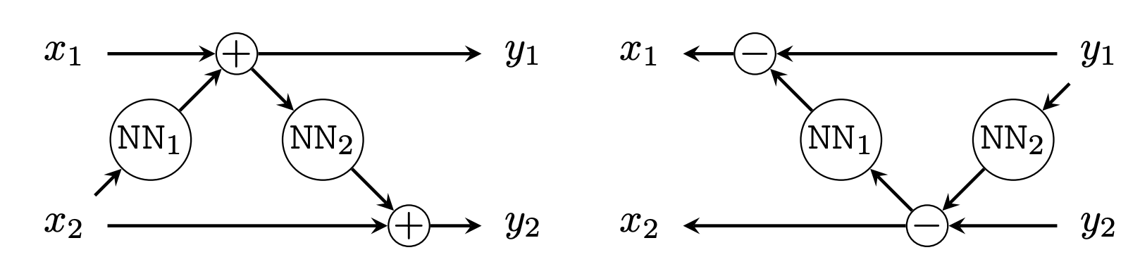

Source: Reversible GANs for Memory-efficient Image-to-Image Translation. This diagramme represents the additive coupling layer in its computation graph form. LEFT: forward pass. RIGHT: reverse pass. To link up the notation $x_1 = \mu_{t}$, $x_2 = x_{t}$, $y_1 = \mu_{t+1}$, $y_2 = x_{t+1}$, $g = \texttt{NN}_1$, and $h=\texttt{NN}_2$

Case study

Specifically in the case of optimisers, I was pointed towards this paper Gradient-based Hyperparameter Optimization with Reversible Learning (2015) by Dougal Maclaurin, David Duvenaud, and Ryan Adams. The authors exploited the reversibility property of SGD with momentum to train the optimiser metaparameters themselves. First they run the optimiser an arbitrary number of steps, say 100 iterations. This defines an optimisation trajectory $x_0, x_1, x_2, …, x_{99}$. Now the clever part is that you can view the unrolled optimisation trajectory as a computation graph in itself. They compute a loss at the end of the trajectory, then they backpropagate the loss in the reverse direction with respect to the optimiser’s metaparameters.

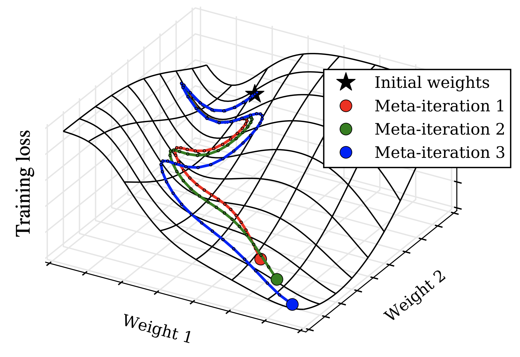
Source: Gradient-based Hyperparameter Optimization with Reversible Learning. The authors optimise metaparameters by backpropagating along optimisation roll outs. This is made possible with the reversibility of momentum-based SGD, to cap memory-complexity.

Could we not do this already, such as in Learning to learn by gradient descent by gradient descent (Andrychowicz et al., 2016)? Well yes, but the crucial point is that you would usually have to store all the intermediate states $\{[x_t, \mu_t]\}_{t=0}^{99}$, which is costly memory-wise. Exploiting the reversibility property, this memory explosion falls away. Indeed there are issues with numerical stability of the inverse, which the papers dives into, but the principle is elegant.

Adam

So what other optimisers are reversible? Let’s consider Adam, where \begin{align} \mu_{t+1} &= \beta_1 \mu_t + (1-\beta_1) \nabla_{x} f(x_{t}) \newline \nu_{t+1} &= \beta_2 \nu_t + (1-\beta_2) (\nabla_{x} f(x_{t}))^2 \newline x_{t+1} &= x_t - \lambda \frac{\mu_{t+1}}{\sqrt{\nu_{t+1}} + \epsilon}. \end{align} Given $x_{t+1}$, $\mu_{t+1}$ and $\nu_{t+1}$, we can easily reconstruct $x_t$ from the last line and from there, we can compute the gradient and recover $\mu_{t}$ and $\nu_{t}$. In maths \begin{align} x_{t} &= x_{t+1} + \lambda \frac{\mu_{t+1}}{\sqrt{\nu_{t+1}} + \epsilon} \newline \mu_{t} &= \frac{1}{\beta_1} \left ( \mu_{t+1} - (1-\beta_1) \nabla_{x} f(x_{t}) \right ) \newline \nu_{t} &= \frac{1}{\beta_2} \left ( \nu_{t+1} - (1-\beta_2) (\nabla_{x} f(x_{t}))^2 \right). \end{align} So Adam is reversible. We actually missed out the bias correction steps \begin{align} \mu_{t+1} &\gets \mu_{t+1} / (1 - \beta_1^{t+1}) \newline \nu_{t+1} &\gets \nu_{t+1} / (1 - \beta_2^{t+1}). \end{align} You can also verify for yourself that these are reversible too.

Do we need reversibility in optimisers?

Well, no. In fact, in some ways, we would rather do without it. Optimisers are supposed to be many-to-one mappings. Starting from an infinity of initial conditions, we should converge to the global minimum of a convex function. This means we should discard information about initialisation along the way. To put it as Maclaurin et al. do:

[O]ptimization moves a system from a high-entropy initial state to a low-entropy (hopefully zero entropy) optimized final state.

It turns out that if you set $\alpha = 0$ for the momentum method; that is, you just run gradient descent, then this is not reversible. I think this may also be true for Nesterov accelerated momentum, and RMSProp which I couldn’t make reversible (I call this proof by fatigue). So I’m left wondering, is reversibility just some extra curious property that can be useful sometimes, but is completely arbitrary when it comes to doing optimisation? Or is there some deeper meaning to it? Is it just some artifact of how we think of optimisation, in terms of balls rolling down hills? Maybe more interestingly, what does the lack of reversibility for standard gradient descent and Nesterov entail? Could this be another reason why Nesterov works better than classical momentum? Could we measure the information loss somehow? And if we could, what would this mean?